How to use the percentage formula in Excel
The percentage calculation feature in Excel makes it easier to calculate percentages. We’ll show you how to use the most important formulas in Excel to calculate percentages of totals or percentage changes such as growth and decline. You’ll also learn how to calculate proportions and totals based on percentages and how to increase and decrease numbers by a percentage.
- Up to 50 GB Exchange email account
- Outlook Web App and collaboration tools
- Expert support & setup service
The basics of calculating percentages in Excel
In this article, we’ll give you an overview of the most important methods for calculating percentages in Excel and show you the most important formulas for doing percentages. The following instructions apply to the Excel version of Microsoft 365 as well as to the 2021, 2019 and 2016 Excel versions.
When you calculate percentages in Excel, you save yourself steps such as multiplying by 100 since the formatting automatically takes care of this for you as soon as you apply the percentage format (see below). The basic Excel percentage calculation formula looks like this:
How to calculate percentages in Excel – Formulas and formatting
Let’s look at a practical example of how percentages are calculated in Excel. A retailer keeps track of their inventory with a spreadsheet. The spreadsheet contains information about the products that they have bought and sold. The number of products that the retailer has bought is in column B, and the number of products that the retailer has sold is in column C. To calculate the percentage of items sold for each product, enter the following formula in the first field of column D (D2):
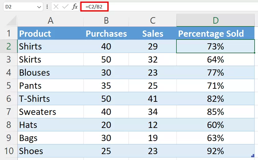
In a formatted table, Excel automatically transfers the percentage formula to the subsequent cells. Alternatively, you can transfer the formula by double-clicking in the bottom right-hand corner of the cell (D2).
Microsoft Excel can make a lot of basic and advanced calculation processes easier, which can be extremely helpful in your everyday work. Learn more about the SUM function in Excel if you are looking for a way to easily add a group of numbers.
Display values in Excel as percentages
The results may not look quite right at first. Instead of percentages, you’ll see decimal numbers in your Excel spreadsheet.
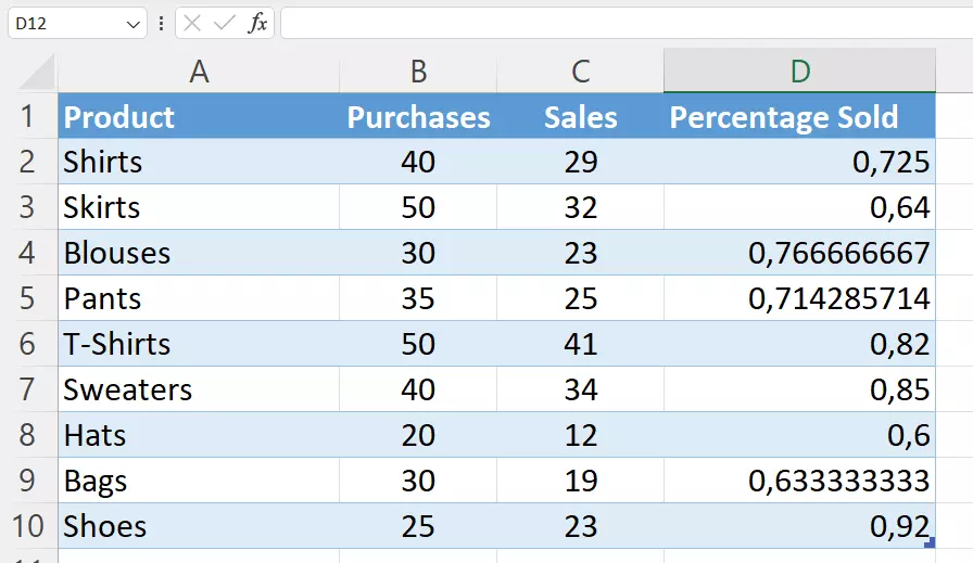
If you want Excel to round the numbers and display the results with the percent sign, you need to change your default settings:
- Click on the Home tab.
- Select the cell range containing the values that should be displayed with a percent sign.
- In the ribbon, click on % in the Number section.
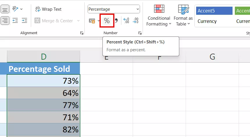
To display values as percents in Excel, you can also use the Excel shortcut[Ctrl] + [Shift] + [%].
Specify percentage with decimal places in Excel
In Excel’s default settings, percentages are displayed without decimal values. However, you can easily change this format by clicking on the small arrow at the bottom right of the Number section. In the Format cells menu that opens, you have the option of specifying how many decimal places should be displayed.
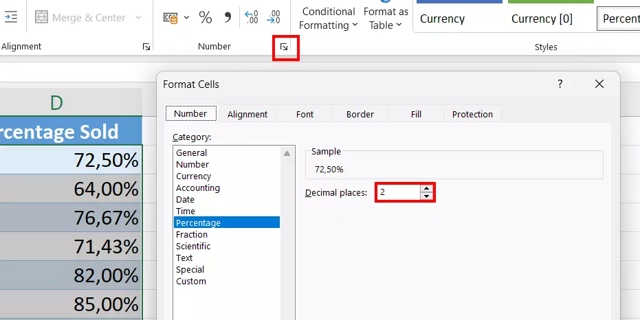
Formatting is not only helpful with percentage calculations in Excel, but with many other processes and tasks as well. For example, in another article in our Digital Guide, you can read about how to calculate time in Excel.
How to calculate the percentage of a sum of values using Excel formulas
In the example above, we calculated percentages based on how many units a retailer had purchased of a specific product, and how many of those units the retailer was able to sell. In the table, purchases represented the total amount, and the sales were the percentages. However, we can also use Excel to do more complex calculations, for example, to find the percentage of a larger amount that is the sum of different values in a table.
Calculating the percentage of a total at the end of an Excel table
Let’s say the retailer in the example above now wants to know how many products they purchased in total, and what the percentage of each individual product is in relation to the total number of products that were purchased. With the help of percentage equations and the right excel formula, you can determine what percentage of the total result each product represents.
First, we need to add an additional cell (our example uses cell B11) to calculate the total amount of products purchased. To do this, we are going to use the formula =SUM(B2:B10).
In column C, we are going to find out what percentage of the total amount of purchases each product represents. To do this, we enter the following formula in cell C2:
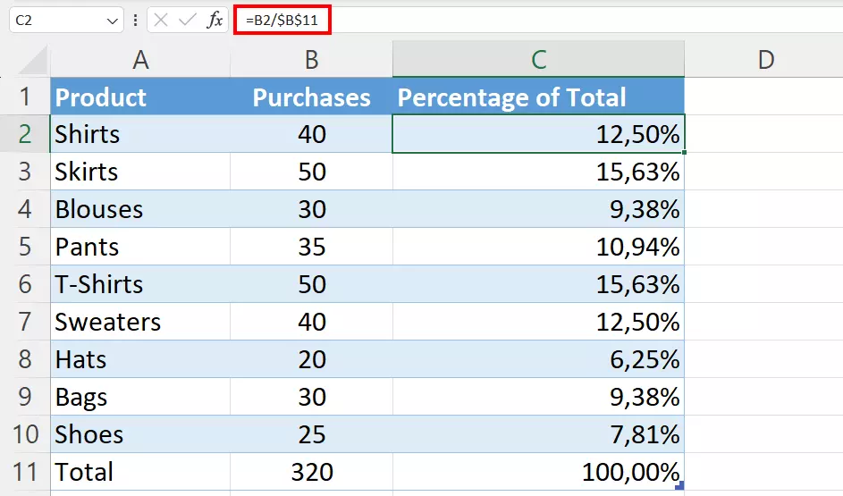
In this case, the $ characters set the absolute reference to cell B11. This means that this value is not changed, even if other values change in the spreadsheet. You can also set a cell as an absolute value by selecting the cell (either with the mouse or by entering it manually) and pressing the [F4] key on your keyboard.
Calculate percentage using values from different rows
Let’s now assume that the retailer has several rows for the same product and wants to use Excel to calculate the percentage that this product accounts for. In this case, you can use Excel SUMIF, which automatically adds all values that match the criterion you have selected. The formula looks like this:
In our example, we entered the criterion Pants in cell E1. The values that we want to add are in column B and the product names for automated selection are in column A. The corresponding formula in Excel is as follows:
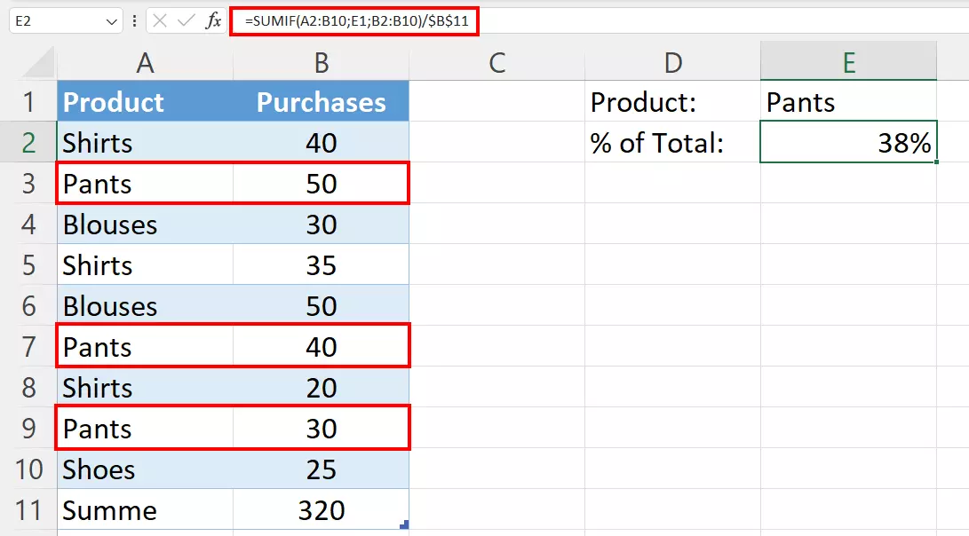
Organize your data in Excel, create spreadsheets and calculate your expenses, profit and much more! Get the spreadsheet software in the Microsoft 365 with setup service from IONOS and benefit from the best support for Excel and other Microsoft software around the clock.
How to use the Excel percentage formula to calculate percentage change
Percentage change or percentage growth is one of the formulas that you’ll probably use most often when calculating percentages in Excel. Simply use the following formula to calculate the change between the original value (A) and another value (B):
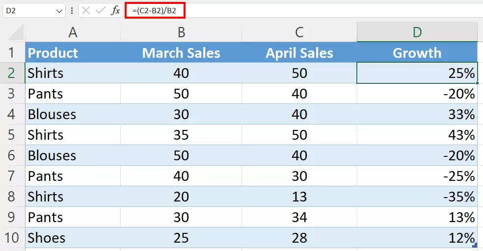
Value (A) represents the value before the change. For example, if you compare sales between March and April, the number of sales in March would be the original value (A) and sales in April would be B. The following two examples illustrate how to calculate the percentage of growth using this formula.
Calculate the percentage change between two columns
The retailer in our example entered the sales from March in column B and the sales from April in column C. The retailer then enters the following formula in column D to calculate the percentage of growth:
- Store, share, and edit data easily
- Backed up and highly secure
- Sync with all devices
Calculate the percentage growth between two rows
You may want to keep track of total monthly sales in a spreadsheet. In this case, you can calculate the percentage growth between two columns so that you can easily see month-over-month changes in sales.
In the example below, we’ve entered all monthly sales in column B and calculated the growth in column C. Start with the sales from January in cell B2 and determine the percentage growth for February in cell C3. To do this, enter the following formula in cell C3:
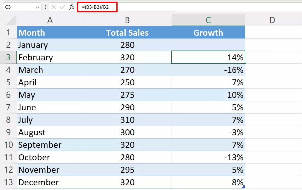
When you calculate the percentage of growth, be sure to leave the first row blank because it is not being used in the comparison. In the example above, January is not compared to the prior month.
How to calculate a total/partial amount in Excel based on a percentage
Just as you can use Excel to calculate a percentage using two values, you can also use Excel to calculate the overall total or a proportion based on a percentage.
Calculate a partial amount
Let’s say you buy new IT equipment for your company and the total price is $1,200. This includes sales tax, which may be tax deductible. Sales tax varies from state to state, so for this example let’s assume that you live in Wisconsin, where sales tax is 5%. For this purpose, you simply calculate the amount of sales tax based on this percentage.
In the following example, the total price is in cell A2 and the percentage is in cell B2. You need to calculate the absolute value of the sales tax in cell C2. Use the following formula:

If you don’t want to enter the percentage in a separate cell, you can also integrate it directly into the formula. Enter either =A2*5% or =A2*0.05.
Calculate a total amount
Excel also allows you to find the total amount of something based on the percentage of a partial amount. For example, let’s say you attend a multi-day workshop in another city. As a workshop attendee, you receive a special discount and pay only 70 percent of the price of your hotel room as part of your all-inclusive accommodation. You are charged $350 and are curious how expensive your stay would have been without the discount.
Enter the amount you paid in cell A2 and the percentage in cell B2. In cell C2, enter the formula for calculating the total price based on the percentage that corresponds to the discount price. Divide your amount by the percentage:

Find out about various other exciting Excel topics in our other articles:

