Wrapping text in Excel: How to display the contents of your Excel cells on multiple lines
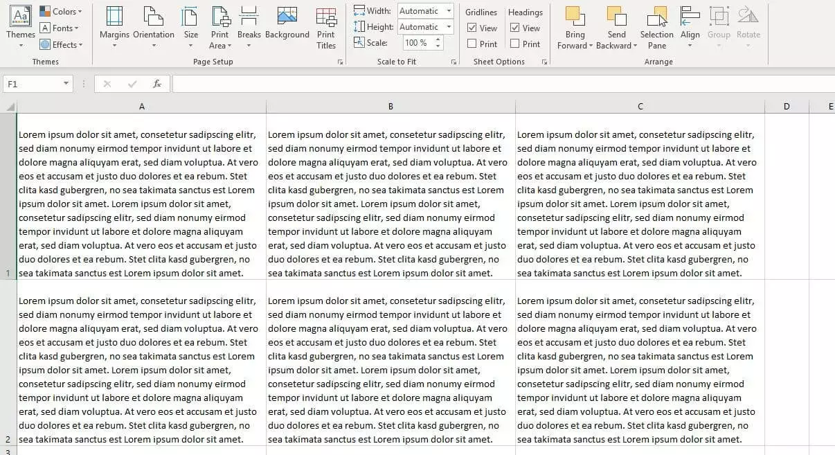
When your Excel spreadsheet has cells with a lot of content, the Microsoft application often displays just a fraction of it and automatically hides the rest. This happens when the length of the text or characters in a cell exceeds the set width of the cell and the neighboring cell is not empty.
You can still view all the contents by double-clicking the cell or selecting the cell and looking in the formula bar, but these methods aren’t very practical. A much more elegant solution is to wrap the text in an Excel cell so that the contents are displayed on multiple lines. We’ll explain how to wrap text in your Excel spreadsheet and deal with any problems you might encounter.
- Store, share, and edit data easily
- Backed up and highly secure
- Sync with all devices
How to wrap text automatically in Excel
The easiest way to wrap text in Excel is to use the automatic text wrap feature. You can enable this feature for any cells in your spreadsheet. When you do this, Excel automatically ensures that the formatted cells contents are displayed on multiple lines so that all the data is visible at all times.
It only takes a few steps to have Excel automatically wrap text in cells: Start by left-clicking the cell that you want to format so that text wraps automatically. If you want to select several cells at once, hold down the left mouse button and then move the mouse over the cells you want to select. Alternatively, hold down the [Ctrl] key and click on the individual cells you want to select:
How to manually enter a line break in Excel
Sometimes it’s useful to have Excel insert a line break at a specific point in a cell, for example if you need to arrange certain content elements underneath each other. Microsoft Excel offers a manual line break function for this purpose. To use it, open Edit mode for the cell you want to edit. You can do this in two ways:
- Double-click the cell.
- Click to select the cell and then press the [F2] key or click in the formula bar.
Now place the cursor where you want Excel to insert the line break in the cell and press the keyboard shortcut [Alt] + [Enter]. Hold down the Alt key.
Use this shortcut twice if you want to insert another line break and add an entire paragraph to the Excel cell (although strictly speaking, there are two line breaks):
Word wrapping not working in Excel: how to fix the problem
The instructions above show how easy it is to wrap text (insert line breaks) in Excel cells. But sometimes the two text wrap functions described above don’t work properly. This often happens when you’re working with third-party Excel documents: Problems with the feature are almost always caused by existing formatting that prevents you from optimizing how lengthy cell contents are displayed. In many cases, the text wrap feature doesn’t work as expected because of the “Merge cells” function or if you’ve set a specific value for the maximum row height.
Solution 1: Clear specific value for row height
In many cases Excel may appear to properly wrap text in a cell, but it still doesn’t show the full contents of the cell. This is usually because the author of the document has set the row to a specific height, which causes Excel to hide some of the content despite the text wrap. You can solve this problem in a few steps:
- Open the “Home” tab.
- Select the problematic cell by left-clicking or right-clicking it.
- In the “Cells” group, click “Format.”
- Choose “AutoFit Row Height.”
Solution 2: Separate merged cells
You can’t wrap text in cells that have been merged in Excel. If manual or automatic wrapping doesn’t work in Excel, it may be because the selected cell is a merged cell. If you want to wrap text in this cell in Excel you must first unmerge the cells.
If you want to keep the merged cell, you can still use the word wrap by manually adjusting the row height and column width.
You can unmerge a merged cell as follows:
- Open the “Home” tab.
- Select the merged cell by left-clicking or right-clicking it.
- In the “Alignment” group, click the drop-down arrow next to “Merge & Center” and then click “Unmerge Cells.”
- Alternatively, if you right-clicked to select the merged cells, you can click “Format cells” and then uncheck the “Merge Cells” checkbox.
- Store, share, and edit data easily
- Backed up and highly secure
- Sync with all devices


