The Excel HLOOKUP function explained in simple terms
The HLOOKUP function in Excel makes it easier to find data located in a predefined table. The “H” in “HLOOKUP” stands for horizontal and refers to the first row of a table. The HLOOKUP function is particularly useful when working with large tables. It eliminates the need to spend a lot of time looking for specific values and provides a result much more quickly. We will explain step by step exactly how to use this practical Excel function for your own needs using a concrete example of HLOOKUP.
When is the Excel HLOOKUP function useful?
Many Excel users work with large amounts of data every day. Maintaining oversight or finding the right information quickly is time consuming and can result in errors. That is why the Microsoft program offers practical reference and lookup functions which can quickly produce the correct results. One such function is HLOOKUP which searches for specific values within a user-defined cell range. It starts the search on the left in the first cell and continues to the right until it reaches the end of the range defined in the function.
HLOOKUP can be used in many situations. For example, imagine that you are selling many different products and want to record your sales in a table at the end of the month. In this situation, it would be tedious to have to look up each product in a price list in order to enter their respective prices individually. Using the Excel HLOOKUP function, you can simply skip this step. The only requirement is that the products in your price list are arranged horizontally. If they are, Excel will enter the prices with the appropriate syntax on its own.
If the values in your table are arranged vertically instead of horizontally, you will need to use the VLOOKUP function. When you use this function, it will perform the search within a column going from top to bottom.
Understanding the syntax of HLOOKUP
To use the HLOOKUP function, you need to understand its syntax and enter it correctly. As with any formula in Excel, even the slightest deviation will result in error messages and incorrect results. However, once you understand how its individual building blocks work, using it is straightforward and will make your work much easier. The following is the basic syntax for the HLOOKUP function in Excel:
The following is what each parameter means:
- The equals sign tells Excel that you are entering a formula in the formula bar instead of a fixed value.
- The lookup_value is a text string or a value that is being searched for. If it is a text string, it must be enclosed in double quotation marks.
- The table_array is the range in your table in which the data is located. This search range can either be selected with the mouse or entered manually.
- The row_index_num indicates which row the result is in. For example, if it is in the fifth row, the row_index_num will be “5”.
- The range_lookup is a logical value that indicates whether you want to find an exact match or an approximate match. If this value is “TRUE”, you will get an approximate match. If it is “FALSE”, you will get an exact match.
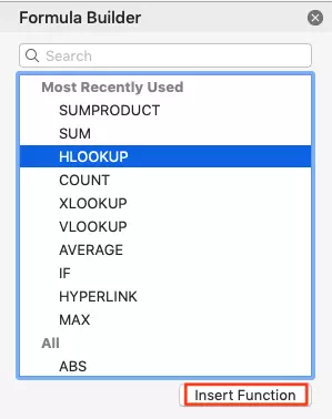
In Excel, you do not need to enter the HLOOKUP syntax manually into the formula bar. Using its formula builder, you can easily enter your important data. You will learn more about the individual steps to do so in the following example.
Practical example of HLOOKUP
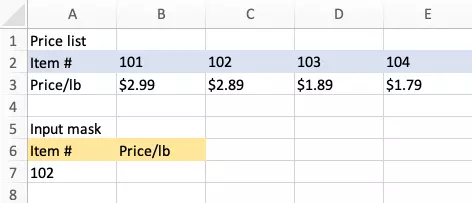
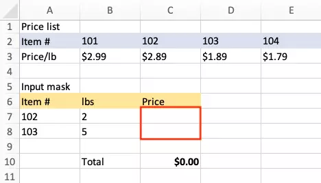
The HLOOKUP function in Excel is particularly useful when you want to look for a specific value in a large data set. This might be a directory with hundreds or thousands of entries. However, a simple example will be enough to get the basic idea across. The image below shows a price list and an input mask.
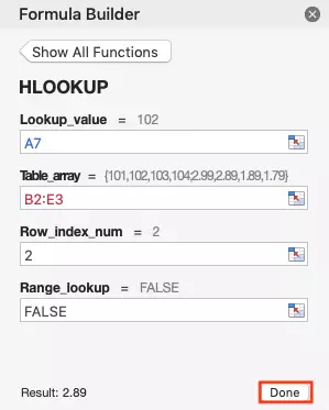
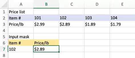
Now, click on “Insert Function” and fill in the entry fields as follows: The lookup_value is A7, which refers to item no. 102, and the table_array extends from B2 to E3. Since the value being looked up is in the second row of the table, the row_index_num is 2. The value under range_lookup is FALSE since only results that match exactly should be displayed.
HLOOKUP: possible combinations with other functions
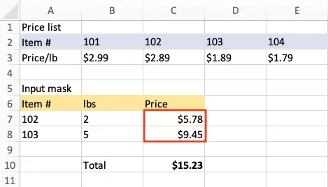
Use the following formulas to multiply the contents of cells B7 and B8 by their corresponding values in the price list and display the results in C7 and C8:
If you want to add the two values together and display the result in C10, you can simply use the SUM function with the table_array defined as C7:C8.


