How to create a table in Excel
When you hear the word Excel, tables are probably what come to mind. With good reason, many people directly associate spreadsheets with the Microsoft software solution. The individual sheets or pages of an Excel spreadsheet resemble tables with their grids of columns and rows. With just a few clicks, you can enter data or import entire datasets into Excel spreadsheets. You can also organize your data into tables without special formatting. However, if you also want to sort, filter, or graphically present your data, formatted tables are your best option.
In the following tutorial we’ll show you how to create a formatted Excel table and tailor it to your needs. We’ll also explain how to remove formatting when you’re done with it.
- Up to 50 GB Exchange email account
- Outlook Web App and collaboration tools
- Expert support & setup service
How to create an Excel table
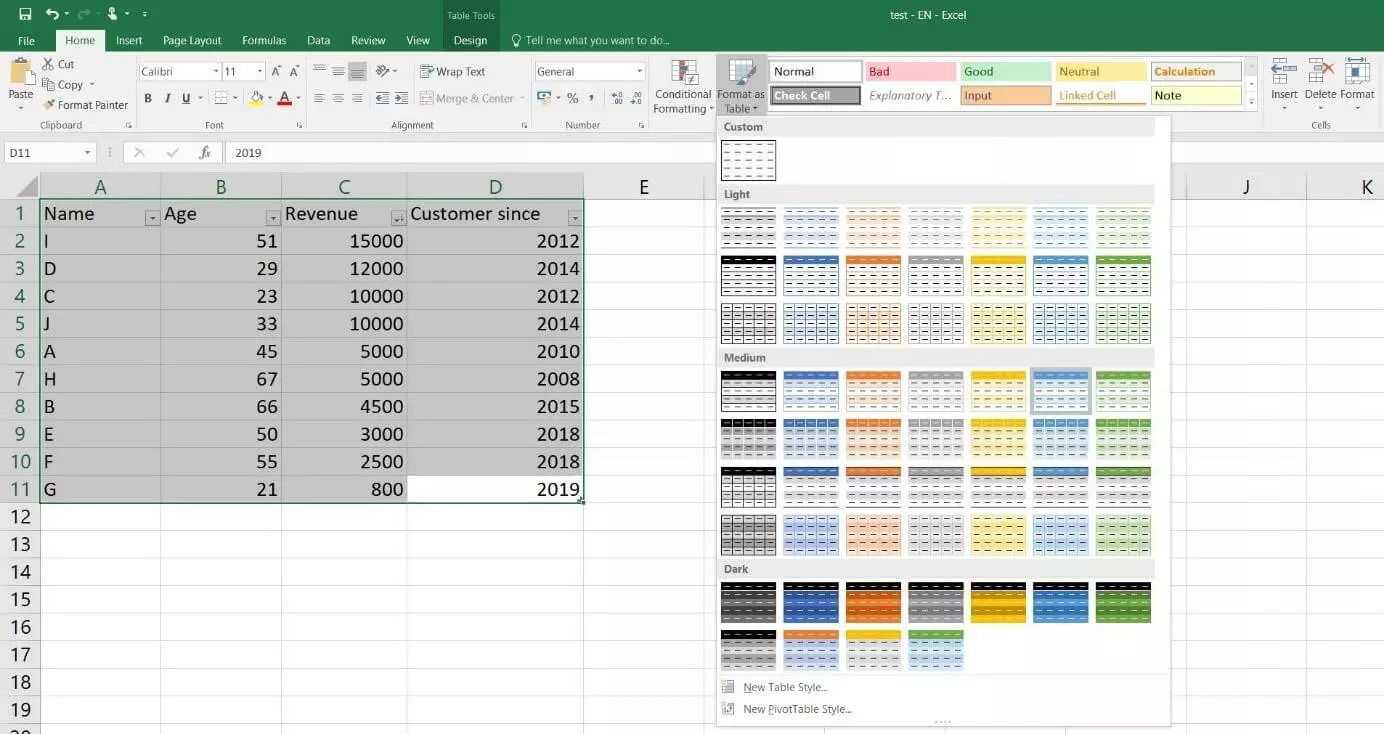
Thanks to a wide range of predefined table styles, you don’t need any special expertise to create formatted Excel tables. If none of the available templates meet your needs, you can easily create your own custom table style. Excel offers a range of options for designing a table format.
Unlike custom table styles, predefined styles for Excel tables cannot be deleted. However, you have the option of clearing both predefined and custom styles. The formatting is then removed and the data is displayed in the default table format.
Integrating or creating a dataset
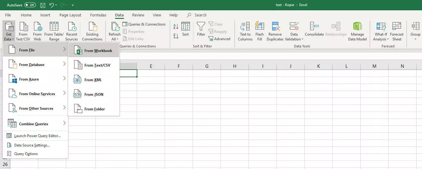
You need a suitable dataset before you can start creating a table. If you want to use features like the filter or sort function, you should also assign appropriate column headers to the data. You can easily integrate data from an external source using the import feature in Excel. To do this, go to the “Data” tab and click the “Get Data” button. Supported import sources include documents (text, CSV, XML, JSON), databases (including Microsoft Access and SQL Server database), Microsoft Azure, and Facebook:
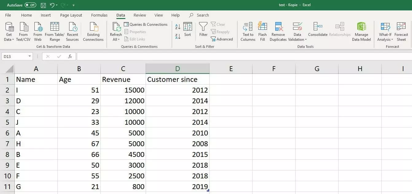
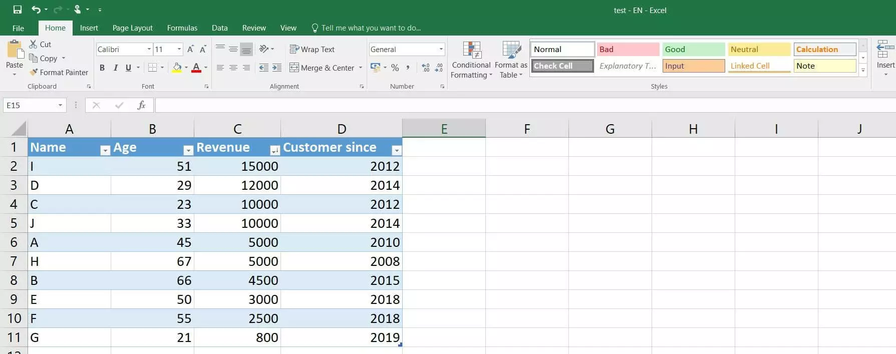
Alternatively, you can manually enter the data for your new Excel table. In the following example, which is also the basis for further steps in this Excel tutorial, we’ve created a small dataset with ten customers. The table lists the name, age, revenue and year of the customer’s first purchase:
Formatting a dataset as a table
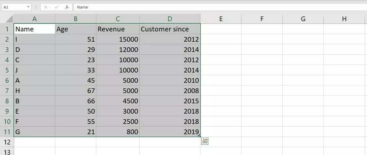
Once you’ve inserted your dataset, you can convert it into a formatted Excel table. To do this, first select the complete dataset by holding down the left mouse button and then selecting all Excel cells you want to convert:
In the dialog box that appears, confirm the dataset cells (in this example, all cells from A1 to D11) and select the “My table has headers” checkbox if you have titled the columns of your dataset. Then click “OK” to create the selected Excel table:
If you haven’t defined titles for your table columns, Excel automatically adds header placeholders to the table during formatting.
Using and removing sort and filter functions
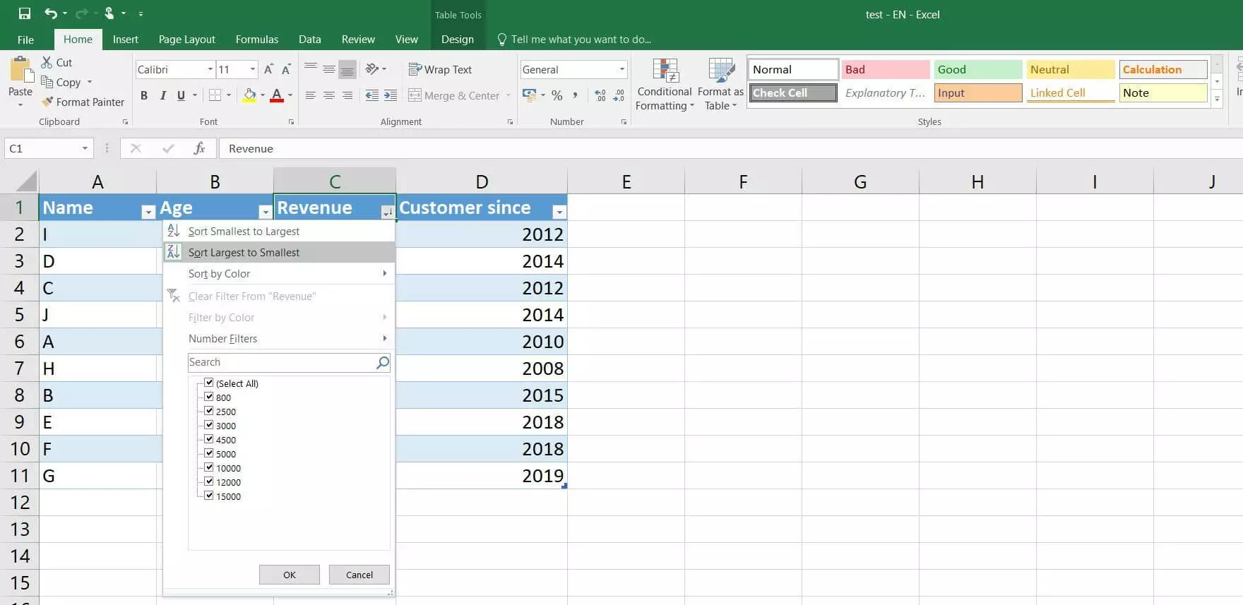
If you create a formatted Excel table for your dataset, Excel adds a sort and filter feature to the table by default. You can use this feature to sort the values of the individual columns alphabetically or numerically or filter them according to your own criteria. To do this, simply click the drop-down arrow icon in the header line of a column and select the option you want to use.
For example, in the Excel table in this tutorial, you can sort customers by revenue (highest to lowest) by clicking the arrow icon in the Sales column and selecting “Sort largest to smallest”:
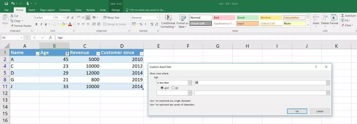
Like the sort function, the filter function automatically differentiates between text and number filters, which you use according to the contents of the column. For example, you can use this feature to display only those customers who are under 50 years old in the Excel table in this tutorial. To do this, choose “Number Filters” and then “Is less than.” In the “Custom AutoFilter” dialog box that appears, enter the value “50” and confirm the filter by choosing “OK”:
If you don’t want to use the filter or the sort function for your Excel table, you can also turn off the feature. First, select one of the cells with the drop-down arrow icon and then click “Sort & Filter” in the upper menu bar (on the Home tab). Then select “Filter” from the drop-down menu to turn off the functions and hide the icons:
Adding a totals row to an Excel table
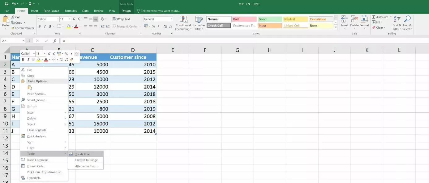
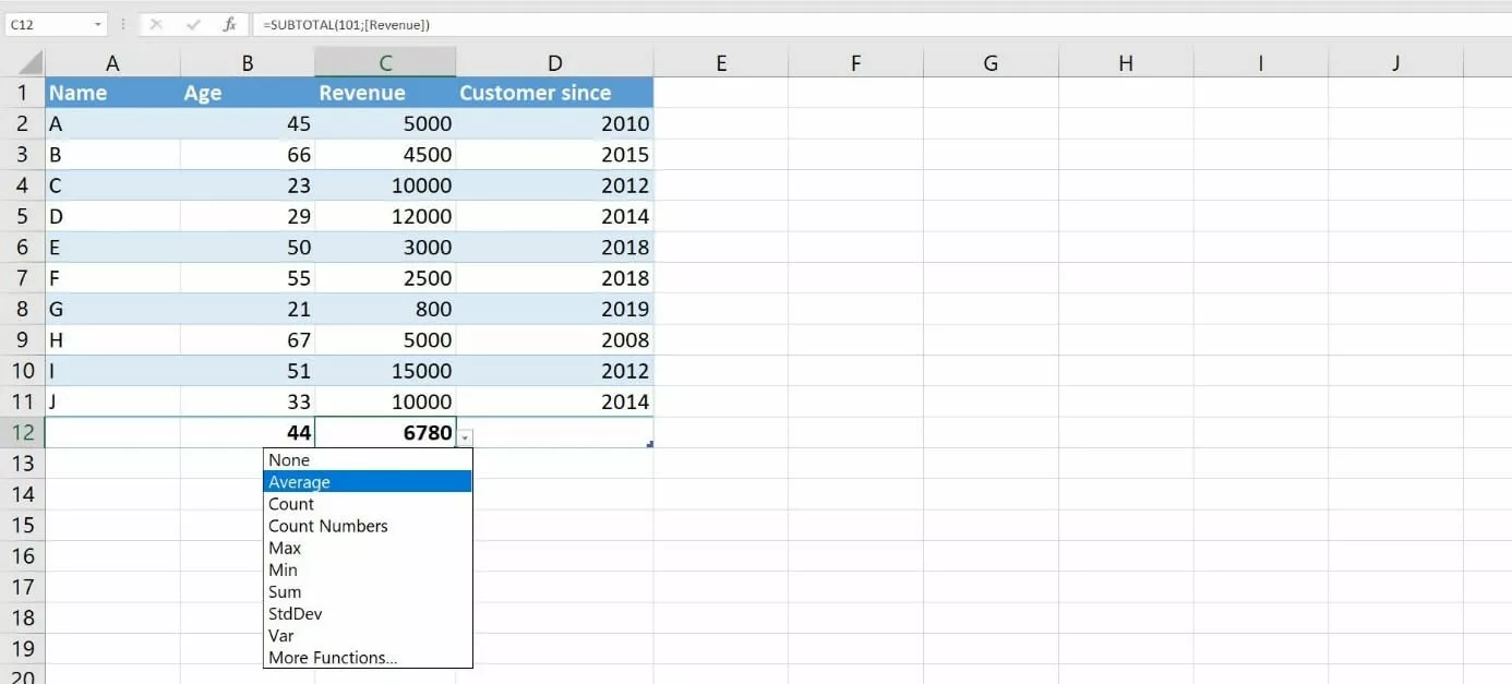
One of the advantages of using a formatted Excel table is that you can add a totals row that automatically presents the results of different calculation options selected from a drop-down list. For example, you can display the sum, the average, specific individual values as well as the minimum or maximum value. To add a total row to your Excel table, simply right-click any cell of the table and select “Table” and then “Totals Row” from the menu:
The totals row uses the familiar drop-down arrow icons. Click this icon in the table column for which you want to select a calculation option. Then select an option to display the result of the calculation in the row. In the following example, we want Excel to calculate the averages for the age and revenue of the customers in the table:
Creating charts from Excel tables
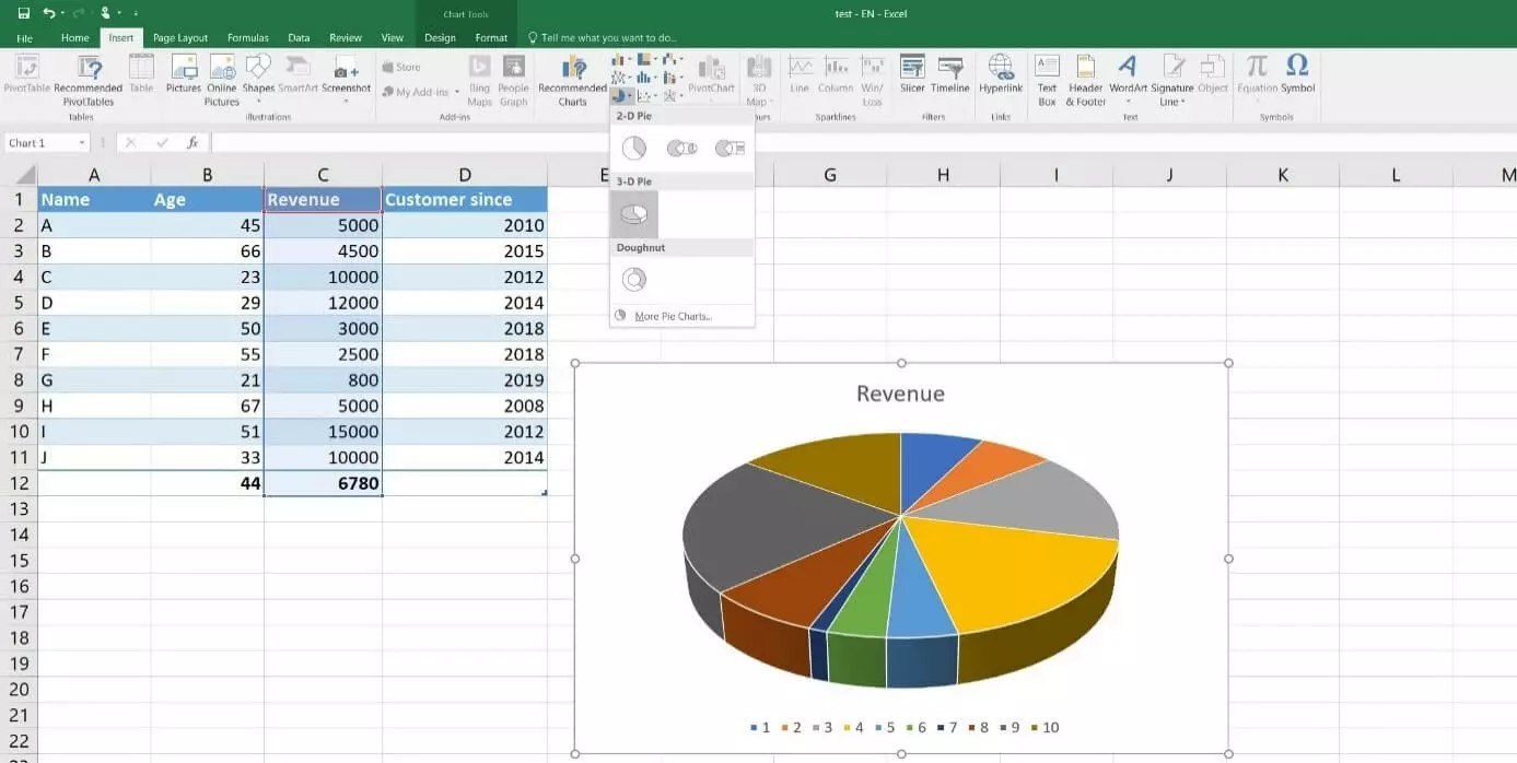
The advantage of creating a formatted Excel table is that you can present the data in charts that are automatically adjusted as you make changes to the table or table values. Follow these steps to create a dynamic chart:
- Open the “Insert” tab.
- Select all rows for which you want to present data in a chart.
- Click “Recommended Charts” in the “Charts” section of the ribbon and select the chart type you want to use. Alternatively, you can click on one of the preselected chart icons.
Removing formatting from an Excel table
If you no longer need certain (or any) formatting in your Excel table or you’ve accidentally formatted cells, you can undo the formatting of these cells at any time. This function is located on the “Home” tab of the ribbon. You can use it as follows:
- Select the cells for which you want to clear the formatting.
- Click the “Clear” button in the “Editing” section.
- Select “Clear Formats” from the drop-down menu.
Excel also has a built-in feature for creating pivot tables. For step-by-step instructions on how to do this, see our detailed how-to article on pivot tables in Excel.
- Up to 50 GB Exchange email account
- Outlook Web App and collaboration tools
- Expert support & setup service
